
Exploratory Data Analysis Project

import pandas as pd
import numpy as np
df = pd.read_csv('Books with genre.csv')
df.head()
| bookID | title | title_desc | Genre_1 | Genre_2 | Genre_3 | authors | average_rating | isbn | isbn13 | language_code | num_pages | ratings_count | text_reviews_count | publication_date | publisher | |
|---|---|---|---|---|---|---|---|---|---|---|---|---|---|---|---|---|
| 0 | 1 | Harry Potter and the Half-Blood Prince | Harry Potter #6) | Fantasy | Young adult literature | Fiction | J.K. Rowling/Mary GrandPré | 4.57 | 439785960 | 9.780000e+12 | eng | 652 | 2095690 | 27591 | 9/16/2006 | Scholastic Inc. |
| 1 | 2 | Harry Potter and the Order of the Phoenix | Harry Potter #5) | Fantasy | Young adult literature | Fiction | J.K. Rowling/Mary GrandPré | 4.49 | 439358078 | 9.780000e+12 | eng | 870 | 2153167 | 29221 | 9/1/2004 | Scholastic Inc. |
| 2 | 4 | Harry Potter and the Chamber of Secrets | Harry Potter #2) | Speculative fiction | Fantasy | Fiction | J.K. Rowling | 4.42 | 439554896 | 9.780000e+12 | eng | 352 | 6333 | 244 | 11/1/2003 | Scholastic |
| 3 | 5 | Harry Potter and the Prisoner of Azkaban | Harry Potter #3) | Fantasy | Speculative fiction | Young adult literature | J.K. Rowling/Mary GrandPré | 4.56 | 043965548X | 9.780000e+12 | eng | 435 | 2339585 | 36325 | 5/1/2004 | Scholastic Inc. |
| 4 | 14 | The Hitchhiker's Guide to the Galaxy | Hitchhiker's Guide to the Galaxy #1) | Science Fiction | Comic novel | Speculative fiction | Douglas Adams | 4.22 | 1400052920 | 9.780000e+12 | eng | 215 | 4930 | 460 | 8/3/2004 | Crown |
df.shape
(2375, 16)
df.info()
<class 'pandas.core.frame.DataFrame'>
RangeIndex: 2375 entries, 0 to 2374
Data columns (total 16 columns):
bookID                2375 non-null int64
title                 2375 non-null object
title_desc            881 non-null object
Genre_1               2375 non-null object
Genre_2               1907 non-null object
Genre_3               1392 non-null object
authors               2375 non-null object
average_rating        2375 non-null float64
isbn                  2375 non-null object
isbn13                2375 non-null float64
language_code         2375 non-null object
num_pages             2375 non-null int64
ratings_count         2375 non-null int64
text_reviews_count    2375 non-null int64
publication_date      2375 non-null object
publisher             2375 non-null object
dtypes: float64(2), int64(4), object(10)
memory usage: 297.0+ KB
df.describe()
| bookID | average_rating | isbn13 | num_pages | ratings_count | text_reviews_count | |
|---|---|---|---|---|---|---|
| count | 2375.000000 | 2375.000000 | 2.375000e+03 | 2375.000000 | 2.375000e+03 | 2375.000000 |
| mean | 19600.002526 | 3.920851 | 9.780067e+12 | 363.136421 | 5.384854e+04 | 1498.799158 |
| std | 13119.490184 | 0.238521 | 8.181855e+08 | 214.242202 | 2.101828e+05 | 4475.537133 |
| min | 1.000000 | 2.820000 | 9.780000e+12 | 0.000000 | 0.000000e+00 | 0.000000 |
| 25% | 8250.500000 | 3.790000 | 9.780000e+12 | 231.000000 | 5.820000e+02 | 49.000000 |
| 50% | 16729.000000 | 3.940000 | 9.780000e+12 | 336.000000 | 5.421000e+03 | 265.000000 |
| 75% | 30245.500000 | 4.080000 | 9.780000e+12 | 449.500000 | 2.709350e+04 | 1049.000000 |
| max | 45572.000000 | 4.570000 | 9.790000e+12 | 1500.000000 | 4.597666e+06 | 94265.000000 |
features = list(df.columns)
list(df.columns) # List of all columns.
['bookID',
 'title',
 'title_desc',
 'Genre_1',
 'Genre_2',
 'Genre_3',
 'authors',
 'average_rating',
 'isbn',
 'isbn13',
 'language_code',
 'num_pages',
 'ratings_count',
 'text_reviews_count',
 'publication_date',
 'publisher']
numeric_features = list(df.describe().columns) # List of numeric columns.
list(df.describe().columns)
['bookID',
 'average_rating',
 'isbn13',
 'num_pages',
 'ratings_count',
 'text_reviews_count']
leftover_features = list(set(features)-set(numeric_features)) # Columns left after removing numeric features.
list(set(features)-set(numeric_features))
['Genre_3',
 'Genre_2',
 'language_code',
 'Genre_1',
 'title',
 'title_desc',
 'publisher',
 'authors',
 'isbn',
 'publication_date']
categorical_features = (df[leftover_features].nunique().loc[df[leftover_features].nunique()<150])._index.to_list()

# Here, we are taking features that have unique values less than 150 to be our categorical features for analysis.
df[leftover_features].nunique()
Genre_3               64
Genre_2               70
language_code          9
Genre_1               98
title               1865
title_desc           800
publisher            656
authors             1235
isbn                2375
publication_date    1262
dtype: int64
df[leftover_features].nunique().loc[df[leftover_features].nunique()<150]
Genre_3          64
Genre_2          70
language_code     9
Genre_1          98
dtype: int64
df[leftover_features].nunique().loc[df[leftover_features].nunique()<150]._index.to_list()
['Genre_3', 'Genre_2', 'language_code', 'Genre_1']
df.isnull().values.any() # Are there any null values?
True
(df.isnull().sum().sum()/np.product(df.shape))*100 # Percentage of null values.
7.75
df.isnull().sum()
bookID                   0
title                    0
title_desc            1494
Genre_1                  0
Genre_2                468
Genre_3                983
authors                  0
average_rating           0
isbn                     0
isbn13                   0
language_code            0
num_pages                0
ratings_count            0
text_reviews_count       0
publication_date         0
publisher                0
dtype: int64
df.isnull().sum().sum()
2945
np.product(df.shape) # df.shape = (2375, 17)
38000
Data Cleaning
df[df.duplicated()] # to check if there are any duplicate rows
| bookID | title | title_desc | Genre_1 | Genre_2 | Genre_3 | authors | average_rating | isbn | isbn13 | language_code | num_pages | ratings_count | text_reviews_count | publication_date | publisher |
|---|
sorted(df['Genre_2'].unique()) # to check for any typographical errors or inconsistent CAPS.
---------------------------------------------------------------------------

TypeError                                 Traceback (most recent call last)

<ipython-input-23-a70f0ddb9afe> in <module>
----> 1 sorted(df['Genre_2'].unique()) # to check for any typographical errors or inconsistent CAPS.


TypeError: '<' not supported between instances of 'float' and 'str'
It shows an error because there is a ‘nan’ values in this column. We will replace that value to ‘Genre Not Mentioned’ for analysis.
df['Genre_2'].fillna('Genre Not Mentioned',inplace=True)
sorted(df['Genre_2'].unique())
['Absurdist fiction',
 'Adventure',
 'Adventure novel',
 'Alternate history',
 'Apocalyptic and post-apocalyptic fiction',
 'Autobiography',
 'Bangsian fantasy',
 'Bildungsroman',
 'Biography',
 "Children's literature",
 'Chivalric romance',
 'Comedy',
 'Comic novel',
 'Conspiracy fiction',
 'Crime Fiction',
 'Detective fiction',
 'Drama',
 'Dystopia',
 'Erotica',
 'Existentialism',
 'Fairytale fantasy',
 'Fantasy',
 'Feminist science fiction',
 'Fiction',
 'Genre Not Mentioned',
 'Gothic fiction',
 'Graphic novel',
 'Historical fiction',
 'Historical novel',
 'Historical whodunnit',
 'Horror',
 'Humour',
 'Inspirational',
 'Juvenile fantasy',
 'Künstlerroman',
 'Literary fiction',
 'Lost World',
 'Magic realism',
 'Mathematics',
 'Memoir',
 'Military science fiction',
 'Morality play',
 'Mystery',
 'Non-fiction',
 'Novel',
 'Novella',
 'Poetry',
 'Politics',
 'Postmodernism',
 'Psychological novel',
 'Psychology',
 'Reference',
 'Religious text',
 'Roman à clef',
 'Romance novel',
 'Satire',
 'Science',
 'Science Fiction',
 'Social criticism',
 'Speculative fiction',
 'Spy fiction',
 'Supernatural',
 'Suspense',
 'Techno-thriller',
 'Time travel',
 'Tragicomedy',
 'True crime',
 'Vampire fiction',
 'War novel',
 'Western',
 'Young adult literature']
df['Genre_3'].fillna('Genre Not Mentioned',inplace=True)
sorted(df['Genre_3'].unique())
['Absurdist fiction',
 'Adventure',
 'Adventure novel',
 'Anti-nuclear',
 'Apocalyptic and post-apocalyptic fiction',
 'Bildungsroman',
 'Biography',
 'Business',
 "Children's literature",
 'Comedy',
 'Comic fantasy',
 'Cozy',
 'Crime Fiction',
 'Detective fiction',
 'Dystopia',
 'Ergodic literature',
 'Erotica',
 'Fantasy',
 'Fiction',
 'Genre Not Mentioned',
 'High fantasy',
 'Historical fiction',
 'Historical novel',
 'Horror',
 'Humour',
 'Inspirational',
 'Künstlerroman',
 'Locked room mystery',
 'Magic realism',
 'Mathematics',
 'Memoir',
 'Military science fiction',
 'Mystery',
 'Nature',
 'Non-fiction',
 'Novel',
 'Novella',
 'Parallel novel',
 'Philosophy',
 'Picaresque novel',
 'Planetary romance',
 'Poetry',
 'Psychological novel',
 'Reference',
 'Religion',
 'Roman à clef',
 'Romance novel',
 'Satire',
 'Science',
 'Science Fiction',
 'Short story',
 'Social science fiction',
 'Social sciences',
 'Sociology',
 'Speculative fiction',
 'Spy fiction',
 'Steampunk',
 'Suspense',
 'Techno-thriller',
 'Travel literature',
 'Utopian and dystopian fiction',
 'War novel',
 'Western fiction',
 'Young adult literature',
 'Zombie']
sorted(df['language_code'].unique())
['en-CA', 'en-GB', 'en-US', 'eng', 'fre', 'ger', 'gla', 'mul', 'spa']
A bird’s-eye view of data!
df['Genre_1'].value_counts().nlargest(10) # Top 10 Genre based on count.
Science Fiction          368
Speculative fiction      332
Fiction                  284
Children's literature    214
Novel                    183
Thriller                 143
Crime Fiction            139
Fantasy                   99
Mystery                   76
Historical fiction        52
Name: Genre_1, dtype: int64
df.groupby('Genre_1')['average_rating'].mean().nlargest(10) # Top 10 Genre based on average rating.
Genre_1
True crime              4.430000
Adventure novel         4.428333
Religious text          4.340000
Self-help               4.300000
Science fantasy         4.240000
Conspiracy fiction      4.220000
Economics               4.180000
Prose poetry            4.145000
Historical fantasy      4.120000
Historical whodunnit    4.120000
Name: average_rating, dtype: float64
df['authors'].value_counts().nlargest(10) # Top 10 Authors based on count
Orson Scott Card       23
Agatha Christie        23
Stephen King           20
Dean Koontz            19
Mercedes Lackey        18
Laurell K. Hamilton    18
Terry Pratchett        18
Robert A. Heinlein     16
Anne Rice              15
Piers Anthony          15
Name: authors, dtype: int64
df['publisher'].value_counts().nlargest(10) # Top 10 Publishers based on count.
Penguin Books               86
Vintage                     86
Penguin Classics            57
Tor Books                   43
Modern Library              40
Ballantine Books            35
Grand Central Publishing    34
Berkley                     34
Bantam                      31
Pocket Books                29
Name: publisher, dtype: int64
df.groupby('title')['average_rating'].mean().nlargest(10) # Top 10 Books based on average rating.
title
Harry Potter and the Half-Blood Prince       4.570
Harry Potter and the Goblet of Fire          4.560
Harry Potter and the Prisoner of Azkaban     4.560
The Lord of the Rings                        4.500
The Return of the King                       4.494
Harry Potter and the Order of the Phoenix    4.490
Lonesome Dove                                4.490
Harry Potter and the Philosopher's Stone     4.470
A Breath of Snow and Ashes                   4.440
Found                                        4.440
Name: average_rating, dtype: float64
df.groupby('title')['ratings_count'].mean().nlargest(10) # Top 10 Books based on no. of ratings.
title
Twilight                                     4597666.0
The Catcher in the Rye                       2457092.0
Harry Potter and the Order of the Phoenix    2153167.0
Animal Farm                                  2111750.0
Of Mice and Men                              1755253.0
The Giver                                    1585589.0
Water for Elephants                          1260027.0
Harry Potter and the Prisoner of Azkaban     1171363.0
Harry Potter and the Chamber of Secrets      1150148.0
The Notebook                                 1090603.0
Name: ratings_count, dtype: float64
Exploratory Data Analysis
import matplotlib.pyplot as plt
import seaborn as sns
%matplotlib inline
sns.set_style('darkgrid')
Numeric Features Distribution
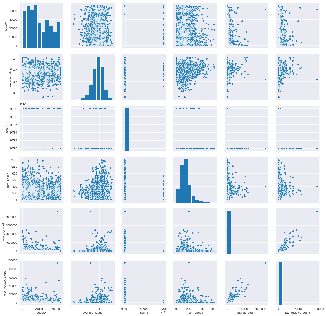
plt.figure(figsize = (12,6))
sns.pairplot(data=df)
<seaborn.axisgrid.PairGrid at 0x27dbf3af048>


<Figure size 864x432 with 0 Axes>
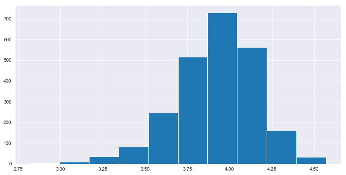
plt.figure(figsize = (12,6))
df['average_rating'].hist() # Distribution of average rating based on count.
<matplotlib.axes._subplots.AxesSubplot at 0x27dc0568080>
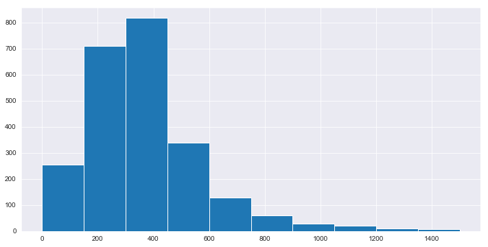
plt.figure(figsize = (12,6))
df['num_pages'].hist() # Distribution of number of pages based on count.
<matplotlib.axes._subplots.AxesSubplot at 0x27dc0136f28>
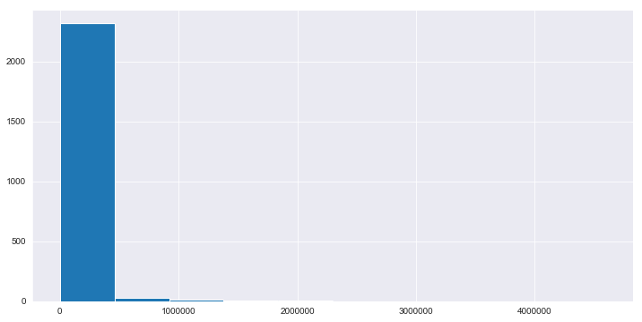
plt.figure(figsize = (12,6))
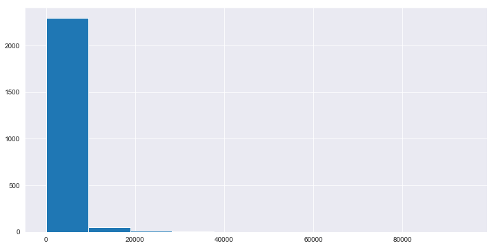
df['ratings_count'].hist() # Distribution of number of ratings based on count.
<matplotlib.axes._subplots.AxesSubplot at 0x27dc0f7a390>
plt.figure(figsize = (12,6))
df['text_reviews_count'].hist() # Distribution of number of text reviews based on count.
<matplotlib.axes._subplots.AxesSubplot at 0x27dc0f7a278>
plt.figure(figsize = (12,6))
sns.countplot(x='Genre_1',data=df)
plt.xticks(rotation=60,horizontalalignment='right')
(array([ 0,  1,  2,  3,  4,  5,  6,  7,  8,  9, 10, 11, 12, 13, 14, 15, 16,
        17, 18, 19, 20, 21, 22, 23, 24, 25, 26, 27, 28, 29, 30, 31, 32, 33,
        34, 35, 36, 37, 38, 39, 40, 41, 42, 43, 44, 45, 46, 47, 48, 49, 50,
        51, 52, 53, 54, 55, 56, 57, 58, 59, 60, 61, 62, 63, 64, 65, 66, 67,
        68, 69, 70, 71, 72, 73, 74, 75, 76, 77, 78, 79, 80, 81, 82, 83, 84,
        85, 86, 87, 88, 89, 90, 91, 92, 93, 94, 95, 96, 97]),
 <a list of 98 Text xticklabel objects>)
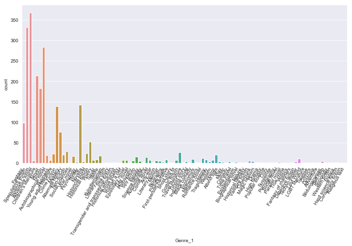
In the above graph we can see that there are a lot of sparse classes (values < 10), so we’ll group them together as OTHER and then view this graph again.
sparse_classes = df['Genre_1'].value_counts()[df['Genre_1'].value_counts() < 10]
df['Filtered_Genre_1'] = df['Genre_1'].apply(lambda x: "OTHER" if x in sparse_classes else x)
# new column to store values of Genre_1 after applying required changes.
plt.figure(figsize = (12,6))
sns.countplot(x='Filtered_Genre_1',data=df)
plt.xticks(rotation=60,horizontalalignment='right')
(array([ 0,  1,  2,  3,  4,  5,  6,  7,  8,  9, 10, 11, 12, 13, 14, 15, 16,
        17, 18, 19, 20, 21, 22, 23, 24]),
 <a list of 25 Text xticklabel objects>)
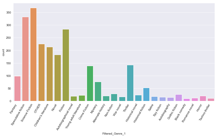
Looks much better! So, the most number of books are ‘Science Fiction’ as Genre_1.
Let’s do the same for Genre_2 and Genre_3..
plt.figure(figsize = (12,6))
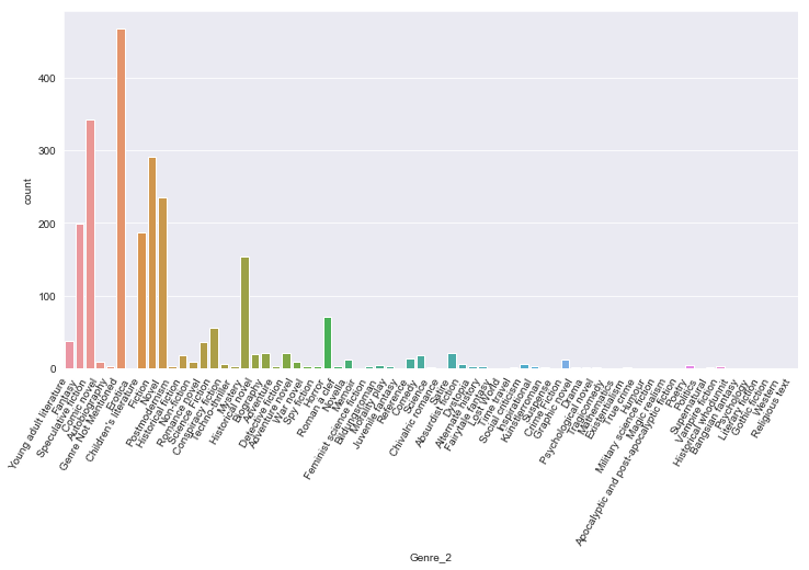
sns.countplot(x='Genre_2',data=df)
plt.xticks(rotation=60,horizontalalignment='right')
(array([ 0,  1,  2,  3,  4,  5,  6,  7,  8,  9, 10, 11, 12, 13, 14, 15, 16,
        17, 18, 19, 20, 21, 22, 23, 24, 25, 26, 27, 28, 29, 30, 31, 32, 33,
        34, 35, 36, 37, 38, 39, 40, 41, 42, 43, 44, 45, 46, 47, 48, 49, 50,
        51, 52, 53, 54, 55, 56, 57, 58, 59, 60, 61, 62, 63, 64, 65, 66, 67,
        68, 69, 70]), <a list of 71 Text xticklabel objects>)
sparse_classes = df['Genre_2'].value_counts()[df['Genre_2'].value_counts() < 10]
df['Filtered_Genre_2'] = df['Genre_2'].apply(lambda x: "OTHER" if x in sparse_classes else x)
# new column to store values of Genre_2 after applying required changes.
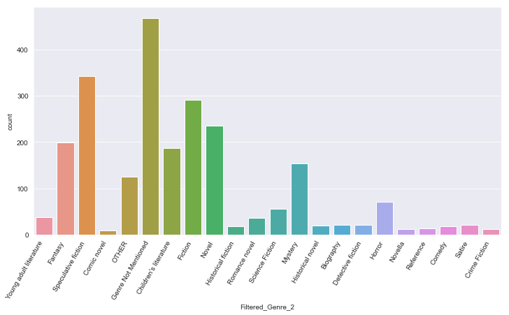
plt.figure(figsize = (12,6))
sns.countplot(x='Filtered_Genre_2',data=df)
plt.xticks(rotation=60,horizontalalignment='right')
(array([ 0,  1,  2,  3,  4,  5,  6,  7,  8,  9, 10, 11, 12, 13, 14, 15, 16,
        17, 18, 19, 20, 21]), <a list of 22 Text xticklabel objects>)
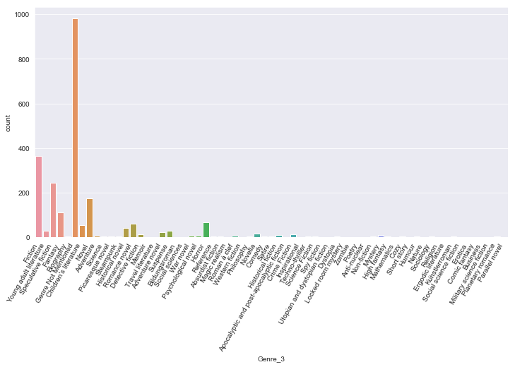
plt.figure(figsize = (12,6))
sns.countplot(x='Genre_3',data=df)
plt.xticks(rotation=60,horizontalalignment='right')
(array([ 0,  1,  2,  3,  4,  5,  6,  7,  8,  9, 10, 11, 12, 13, 14, 15, 16,
        17, 18, 19, 20, 21, 22, 23, 24, 25, 26, 27, 28, 29, 30, 31, 32, 33,
        34, 35, 36, 37, 38, 39, 40, 41, 42, 43, 44, 45, 46, 47, 48, 49, 50,
        51, 52, 53, 54, 55, 56, 57, 58, 59, 60, 61, 62, 63, 64]),
 <a list of 65 Text xticklabel objects>)
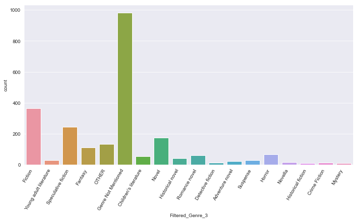
sparse_classes = df['Genre_3'].value_counts()[df['Genre_3'].value_counts() < 10]
df['Filtered_Genre_3'] = df['Genre_3'].apply(lambda x: "OTHER" if x in sparse_classes else x)
# new column to store values of Genre_3 after applying required changes.
plt.figure(figsize = (12,6))
sns.countplot(x='Filtered_Genre_3',data=df)
plt.xticks(rotation=60,horizontalalignment='right')
(array([ 0,  1,  2,  3,  4,  5,  6,  7,  8,  9, 10, 11, 12, 13, 14, 15, 16,
        17]), <a list of 18 Text xticklabel objects>)
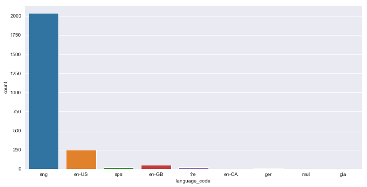
plt.figure(figsize = (12,6))
sns.countplot(x='language_code',data=df)
<matplotlib.axes._subplots.AxesSubplot at 0x27dc267d198>
Now, let’s create a new column ‘Group_genre’ with combined values from Genre_1, Genre_2 and Genre_3.
df['Group_genre'] = df['Filtered_Genre_1']+' / '+df['Filtered_Genre_2']+' / '+df['Filtered_Genre_3']
plt.figure(figsize = (12,6))
sns.countplot(x='Group_genre',data=df)
<matplotlib.axes._subplots.AxesSubplot at 0x27dc2a35d30>
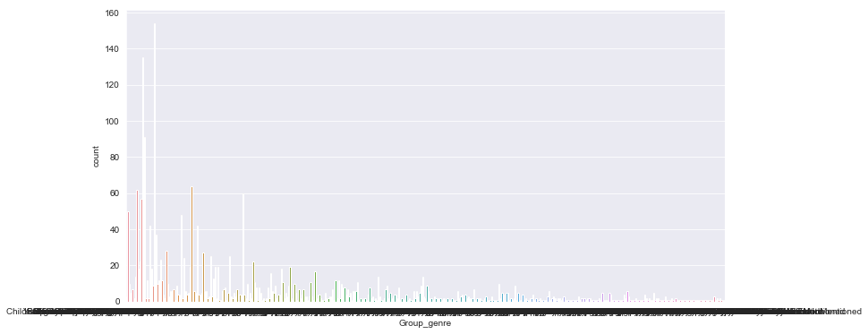
sparse_classes = df['Group_genre'].value_counts()[df['Group_genre'].value_counts() < 10]
df['Filtered_Group_genre'] = df['Group_genre'].apply(lambda x: "OTHER" if x in sparse_classes else x)
# new column to store values of Group_genre after applying required changes.
plt.figure(figsize = (12,6))
sns.countplot(x='Filtered_Group_genre',data=df)
plt.xticks(rotation=60,horizontalalignment='right')
(array([ 0,  1,  2,  3,  4,  5,  6,  7,  8,  9, 10, 11, 12, 13, 14, 15, 16,
        17, 18, 19, 20, 21, 22, 23, 24, 25, 26, 27, 28, 29, 30, 31, 32, 33,
        34, 35, 36, 37, 38, 39, 40, 41, 42, 43, 44, 45, 46, 47, 48, 49]),
 <a list of 50 Text xticklabel objects>)
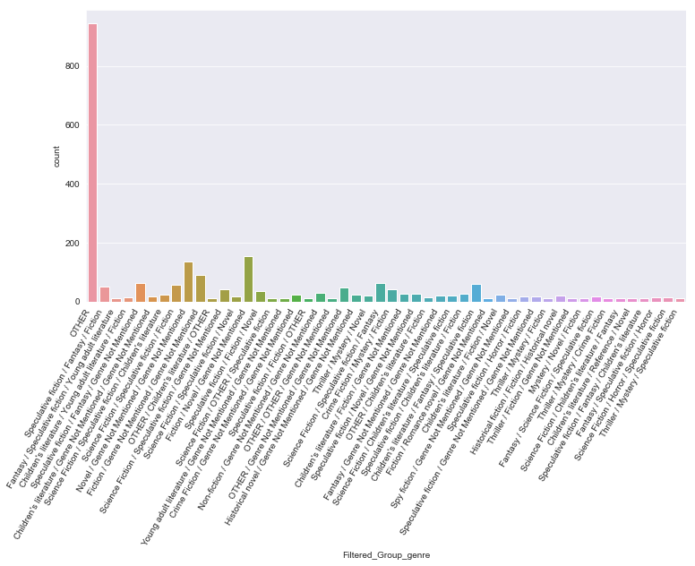
It wasn’t very useful I guess, but I am just learning! :)
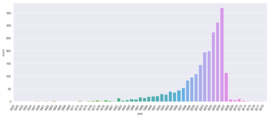
Let’s analyse the date field.
df['publication_date'] = pd.to_datetime(df['publication_date']) # date field coverted from str to datetime
df['year'] = df['publication_date'].apply(lambda x: x.year)
df['month'] = df['publication_date'].apply(lambda x: x.month)
# year and month derived from the date field.
plt.figure(figsize = (15,6))
sns.countplot(x='year',data=df)
plt.xticks(rotation=60,horizontalalignment='right')
# plot of number of books per year.
(array([ 0,  1,  2,  3,  4,  5,  6,  7,  8,  9, 10, 11, 12, 13, 14, 15, 16,
        17, 18, 19, 20, 21, 22, 23, 24, 25, 26, 27, 28, 29, 30, 31, 32, 33,
        34, 35, 36, 37, 38, 39, 40, 41, 42, 43, 44, 45, 46, 47, 48, 49, 50,
        51, 52, 53, 54, 55, 56, 57, 58]),
 <a list of 59 Text xticklabel objects>)
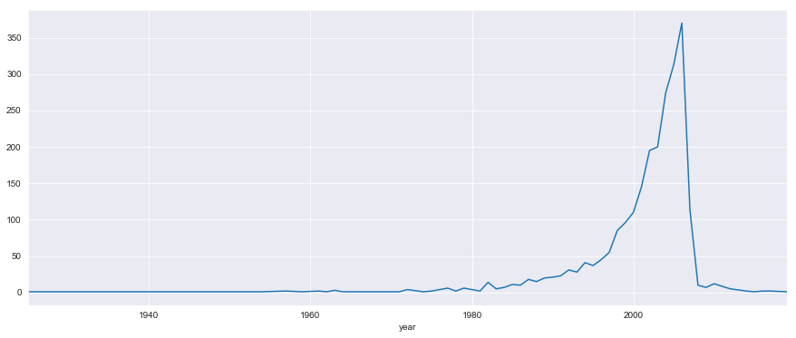
byyear = df.groupby('year').count()
byyear.head()
| bookID | title | title_desc | Genre_1 | Genre_2 | Genre_3 | authors | average_rating | isbn | isbn13 | ... | ratings_count | text_reviews_count | publication_date | publisher | Filtered_Genre_1 | Filtered_Genre_2 | Filtered_Genre_3 | Group_genre | Filtered_Group_genre | month | |
|---|---|---|---|---|---|---|---|---|---|---|---|---|---|---|---|---|---|---|---|---|---|
| year | |||||||||||||||||||||
| 1925 | 1 | 1 | 0 | 1 | 1 | 1 | 1 | 1 | 1 | 1 | ... | 1 | 1 | 1 | 1 | 1 | 1 | 1 | 1 | 1 | 1 |
| 1940 | 1 | 1 | 0 | 1 | 1 | 1 | 1 | 1 | 1 | 1 | ... | 1 | 1 | 1 | 1 | 1 | 1 | 1 | 1 | 1 | 1 |
| 1952 | 1 | 1 | 1 | 1 | 1 | 1 | 1 | 1 | 1 | 1 | ... | 1 | 1 | 1 | 1 | 1 | 1 | 1 | 1 | 1 | 1 |
| 1953 | 1 | 1 | 0 | 1 | 1 | 1 | 1 | 1 | 1 | 1 | ... | 1 | 1 | 1 | 1 | 1 | 1 | 1 | 1 | 1 | 1 |
| 1954 | 1 | 1 | 0 | 1 | 1 | 1 | 1 | 1 | 1 | 1 | ... | 1 | 1 | 1 | 1 | 1 | 1 | 1 | 1 | 1 | 1 |
5 rows × 22 columns
plt.figure(figsize = (15,6))
byyear['bookID'].plot()
# continous distribution of number of books yearly.
<matplotlib.axes._subplots.AxesSubplot at 0x27dc37629b0>
plt.figure(figsize = (12,6))
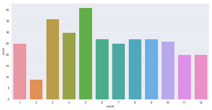
byyear = df[df['year']==2005]
sns.countplot(x='month',data=byyear)
# Month-wise number of books of year 2005. Similarly we can see for other years.
<matplotlib.axes._subplots.AxesSubplot at 0x27dc3f86e48>
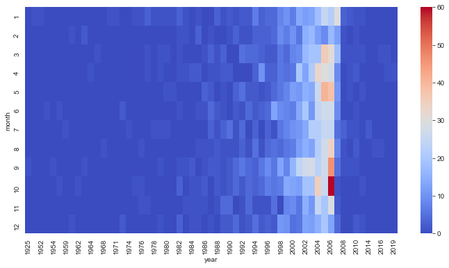
monthyear = df.groupby(by=['month','year']).count()['bookID'].unstack()
monthyear.fillna(0,inplace=True)
monthyear.head()
| year | 1925 | 1940 | 1952 | 1953 | 1954 | 1957 | 1959 | 1961 | 1962 | 1963 | ... | 2007 | 2008 | 2009 | 2010 | 2012 | 2014 | 2015 | 2016 | 2017 | 2019 |
|---|---|---|---|---|---|---|---|---|---|---|---|---|---|---|---|---|---|---|---|---|---|
| month | |||||||||||||||||||||
| 1 | 0.0 | 1.0 | 1.0 | 0.0 | 0.0 | 0.0 | 0.0 | 0.0 | 0.0 | 0.0 | ... | 30.0 | 3.0 | 2.0 | 1.0 | 1.0 | 0.0 | 0.0 | 0.0 | 0.0 | 0.0 |
| 2 | 0.0 | 0.0 | 0.0 | 0.0 | 0.0 | 0.0 | 0.0 | 1.0 | 0.0 | 2.0 | ... | 12.0 | 1.0 | 0.0 | 1.0 | 0.0 | 0.0 | 0.0 | 0.0 | 0.0 | 0.0 |
| 3 | 0.0 | 0.0 | 0.0 | 0.0 | 0.0 | 0.0 | 0.0 | 0.0 | 0.0 | 0.0 | ... | 18.0 | 1.0 | 1.0 | 1.0 | 1.0 | 0.0 | 0.0 | 1.0 | 1.0 | 0.0 |
| 4 | 0.0 | 0.0 | 0.0 | 0.0 | 0.0 | 0.0 | 0.0 | 0.0 | 0.0 | 0.0 | ... | 9.0 | 0.0 | 1.0 | 2.0 | 0.0 | 0.0 | 0.0 | 0.0 | 1.0 | 1.0 |
| 5 | 0.0 | 0.0 | 0.0 | 0.0 | 0.0 | 0.0 | 0.0 | 0.0 | 0.0 | 0.0 | ... | 11.0 | 0.0 | 1.0 | 0.0 | 1.0 | 0.0 | 0.0 | 0.0 | 0.0 | 0.0 |
5 rows × 59 columns
plt.figure(figsize = (12,6))
sns.heatmap(monthyear,cmap='coolwarm')
#This heatmap shows a relationship between the number of books per month year-wise.
<matplotlib.axes._subplots.AxesSubplot at 0x27dc3da43c8>
plt.figure(figsize = (12,6))
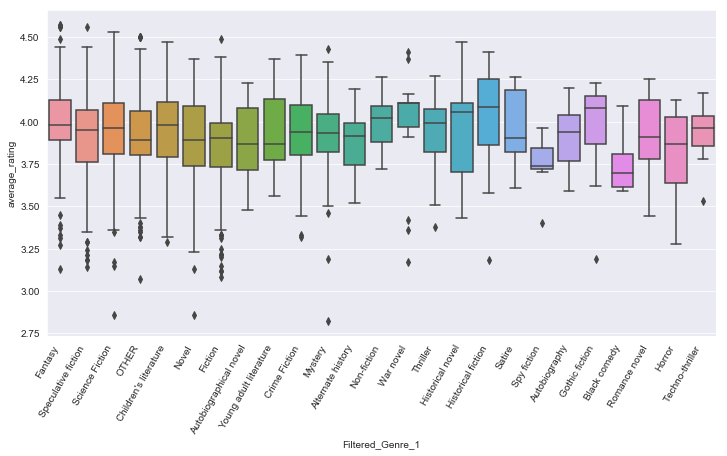
sns.boxplot(x='Filtered_Genre_1',y='average_rating',data=df)
plt.xticks(rotation=60,horizontalalignment='right')
#This shows a relationship between Genre and the average rating.
(array([ 0,  1,  2,  3,  4,  5,  6,  7,  8,  9, 10, 11, 12, 13, 14, 15, 16,
        17, 18, 19, 20, 21, 22, 23, 24]),
 <a list of 25 Text xticklabel objects>)
plt.figure(figsize = (12,6))
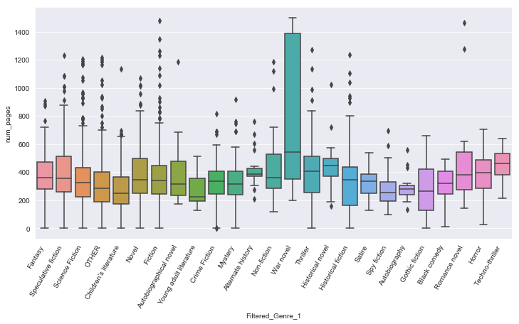
sns.boxplot(x='Filtered_Genre_1',y='num_pages',data=df)
plt.xticks(rotation=60,horizontalalignment='right')
#This shows a relationship between Genre and the number of pages.
(array([ 0,  1,  2,  3,  4,  5,  6,  7,  8,  9, 10, 11, 12, 13, 14, 15, 16,
        17, 18, 19, 20, 21, 22, 23, 24]),
 <a list of 25 Text xticklabel objects>)
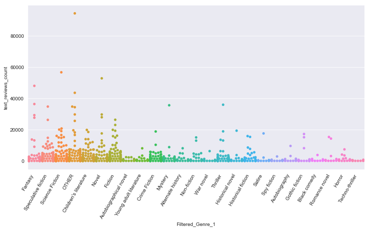
plt.figure(figsize = (12,6))
sns.swarmplot(x='Filtered_Genre_1',y='text_reviews_count',data=df)
plt.xticks(rotation=60,horizontalalignment='right')
#This shows a relationship between Genre and the number of text reviews.
(array([ 0,  1,  2,  3,  4,  5,  6,  7,  8,  9, 10, 11, 12, 13, 14, 15, 16,
        17, 18, 19, 20, 21, 22, 23, 24]),
 <a list of 25 Text xticklabel objects>)
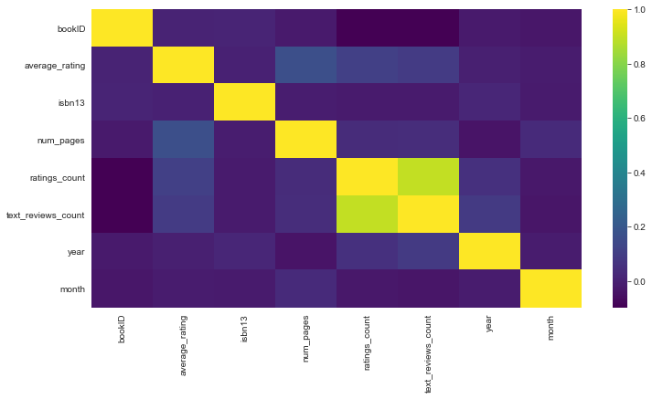
plt.figure(figsize = (12,6))
sns.heatmap(df.corr(),cmap='viridis')
# This heatmap shows the dependencies existing between numeric features.
<matplotlib.axes._subplots.AxesSubplot at 0x27dc572f160>
This completes Exploratory Data Analysis. :)